The tire model RB (Rigid Belt) simplifies, in principle, the tire belt into a rigid belt body, which is defined by a radius and a belt width. Meanwhile, the tire model RB describes the contact between the tire model and the contact area by cutting a parametrizable geometry with the ground layer or description of the ground model.
THEORY OF THE MODEL IN BRIEF
The interface between vehicle model and tyre mode
Numerical Treatment
RMOD-K 7 is a software system, based on some new theoretical work in the field of dynamics of rolling systems. The development of RMOD-K 7 was strongly influenced by the users group of RMOD-K, from where a lot of hints and wishes came. This text describes the properties and the use of the rigid ring belt model (RFNRB), which can be used up to frequencies of approximately 100 Hz and ground disturbance wavelengths about 100 Millimeters. Because of some new modeling approaches, not all model parameters have the same meaning and some new parameters where introduced, mainly to improve the accuracy in the field of tyre characteristics (steady state tyre behavior).
Together with RMOD-K 7 comes a new small MBS system called RMOD-M(otion). RMOD-M is a stand-alone system, which can be used to calculate the steady state tyre behavior (forces versus slip) or to calculate the sweep slip responses of a certain type of tyre to get some insights into the tyre behavior in the frequency domain. RMOD-M runs independent from any commercial MBS-Code, because the equations the motion of rim and belt are solved inside RMOD-M using a stiff integrator.
There are three major differences in the theory of RMOD-K 7 with respect to earlier versions, the interfacing, the numerical treatment of the partial differential equations of tangential contact and the description of the contact area.
The interface between vehicle model and tyre model
The belt is regarded as rigid part in RFN-RB and used to represent the modes of vibration and to calculate the field of velocities in the contact area. Possible interfaces between tyre and vehicle are shown in table 1.
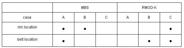
Table 1: possible interfaces between vehicle and tyre
While in case C, rim and belt are regarded as part of the tyre model, in case A both parts belong to the vehicle model. Case B shows the interface of RMOD-K 6.x. Because of the rigid belt in this class of tyre models, using an interface as shown in case A offers a lot of advantages.
- Numerical treatment of the belt’s equation of motion is done by the MBS integrator, so the MBS integrator knows the corresponding frequencies of the belt modes. In consequence, the Jacobeans of the entire system of vehicle and tyre are more accurate and easier to obtain.
- Linearization and vibration analyses can by carried out using the MBS procedures without any changes of the interface. Couplings between belt/rim and suspension vibrations can be investigated more easily.
- Numerical stability of critical parts as for instance the rim at nondriven wheels is improved. The degrees of freedom of the belt can be chosen the respect to the simulation task and can be change even during the simulation.
- The deformation and vibration of the belt can be visualized in the MBS postprocessor if there is some geometry for the belt.
The connection between the belt and the rim can be done in different ways, all representing a special kind of tyre model.
- Fixed joint between belt and rim: all degrees of freedom of the belt are constraint, so the belt’s natural frequencies will not influence the motion or the numerical integration. This may be used, if only the state steady vehicle behavior is investigated or the highest frequencies of the systems are less than 20 Hz. Then, the only dynamic element in RMOD-K is the contact.
- Planar joint and bushing between belt and rim: some of the belt’s degrees of freedom are constraint, for instance the belt rotation about the rim axis and the deflections in longitudinal direction as well as normal to the road are free, the bushing parameters and the belts inertias can be derived from an RMOD-M run. This may be used, when the vehicle behavior while braking straight ahead is of interest.
- Bushing element between belt and rim: none of the belt’s degrees of freedom are constraint, the bushing parameters and the belt’s inertias can be derived from an RMOD-M run.
RMOD-M provides bushing stiffness and damping data as well as mass and inertia of the belt. Because the belt is treated as symmetric body, stiffness and damping in x and z direction are equal, if y is the rim axis of revolution as for instance in figure 1.
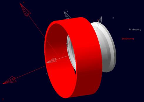
Figure 1: belt and rim bushing marker
DATAFILE rfn20.225
BUSHING AND BELT PART DATA X Y Z
TRANSLATIONAL STIFFNESS [N/mm] 0.612684E+04 0.143211E+04 0.612684E+04
TRANSLATIONAL DAMPING [Ns/mm] 0.757528E+00 0.319489E+00 0.757528E+00
ROTATIONAL STIFFNESS [Nmm/rad] 0.424320E+09 0.225429E+10 0.424320E+09
ROTATIONAL DAMPING [Nsmm/rad] 0.764872E+05 0.431754E+06 0.764872E+05
ROTATIONAL STIFFNESS [Nmm/deg] 0.243117E+11 0.129161E+12 0.243117E+11
ROTATIONAL DAMPING [Nsmm/deg] 0.438240E+07 0.247377E+08 0.438240E+07
BELT INERTIAS [Ns^2 mm] 0.205049E+04 0.410097E+04 0.205049E+04
BELT MASS [Ns^2/mm] 0.106000E-01
Table 2: RMOD-M outputfile BELTBUSH.DAT
To convert an MBS model to RMOD-K 7, the user has only to generate a new part, a bushing and some markers. The structure of the interface between MBS and RMOD-K 7 is the same as in earlier version, so the requirements as orientation and position of reference markers, number of strings and so on remains unchanged.
The RMOD-K output file BELTBUSH.DAT contains the information of table 2. If the orientation of the belt- and rim bushing marker are different to that of figure 2, then the data of table 2 has to be change accordingly.
The dynamics of contact is given by the first order partial differential equations for the displacements in the contact area:
u and v are the displacements while VT is the transport velocity gv(x,t) and gu(x,t) are the slip velocities. The partial differential equations are not coupled in the case of sticking, coupling takes place only when sliding occurs. In RMOD-K 7, these equations are solved with a stiff integration method, which enlarges the regions of stability widely. Nonstiff methods have small regions of stability as shown in figure 2 and therefore the MBS step width is limited because of the limitations in the tyre model. In figure 2, the light gray lines show the eigenvalues of contact with respect to the number of contact points while the black lines show the stable regions of a Runge-Kutta method (DOPRI) for different step sizes dt.
Figure 2: regions of stability and eigenvalues of contact wrt. number of contact points
In RMOD-K 7, the solver is a BDF solver, which can be reduced to an order N algorithm for each direction in u and v. It is shown in [1] that the new integration method is absolute stable in the case of total sticking and a linear system. When sliding occurs, the numerical stability is no longer absolute, but the region of stability remains much larger than with explicit methods.
Contact and belt dynamics of the tyre lead to complex force distributions in the contact area. The model is able to generate information concering this as animations of the stresses, the velocities and other like stick/slip status. From the longitudinal force distribution in Figure 3, the border between sticking and sliding area can be seen.
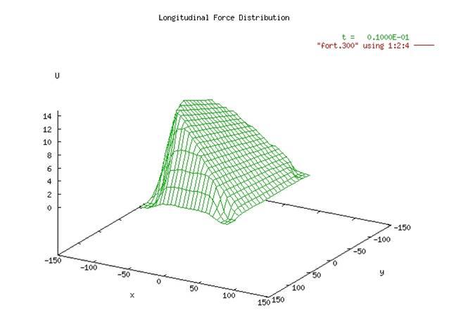
Figure 3: longitudinal forces distribution
Dynamic inputs from yaw, camber and wheel load lead to the results shown in Figure 4. The lateral slip magnitude is 10 [deg] at 1 [Hz] together with a camber angle variation of 3 [deg] at 1 [Hz] and a wheel load variation 3000-5000 [N] at 0.25 [Hz].
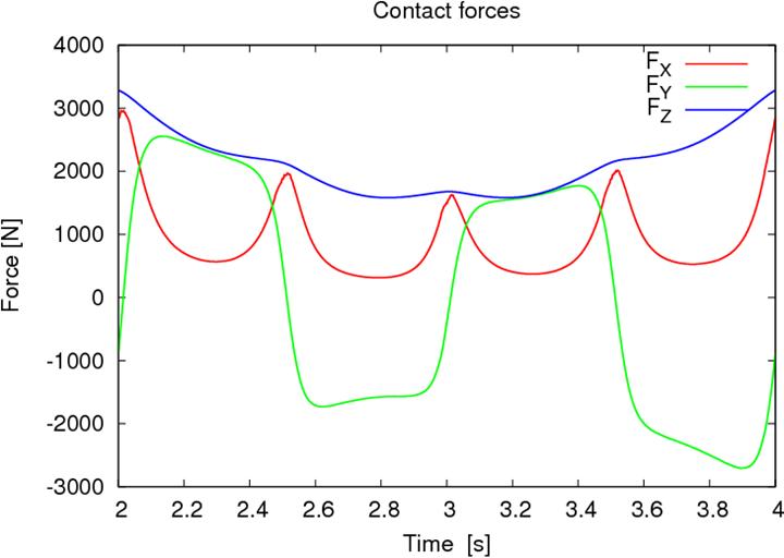
Figure 4: rim force, dynamic inputs from yaw, camber and wheel load
Because the rigid belt model contains now calculation of the tyre’s structure dynamics, approximations are used to get the shape of the contact area and the pressure distribution. In consequence, not all of the parameters are physical, there remain some approximation parameters. These parameters must be determined by comparing the measured tyre properties as for instance steady state tyre forces. Also, the friction values on different tracks are not available always, so some justifications may be necessary. The parameters of RFNRB may be grouped as follows
- grid parameters that define the numbers of grid points (dynamic and refine),
- belt dynamics parameters defining the eigenvalues and damping of the belt,
- geometry parameters of the approximation of the contact area’s shape,
- parameters of the approximation of the pressure distribution,
- parameters influencing the tyre’s slip stiffness in the sticking area and
- parameters that determine the tyre characteristics in sliding area.
In table 2 in the appendix, all parameters used in the input deck of RFNRB (for instance a file named 'MYRFN20.225') in RMOD-K 7 are explained; some default values and ranges are given. The user may use RMOD-M to study the influence of individual parameters on the calculated tyre behavior.